2D data(image)의 경우에는 ORB, SIFT, HOG등등의 descriptor들을 들어봤는데 3D data에 대해서는 제대로 알아본적이 없어서 A comprehensive review of 3D point cloud descriptors 라는 제목의 review 논문 + 여러 pointcloud 관련 task를 적용한 논문들을 통해서 알아보고자 하였다. 각각의 방법론의 소제목 옆에 있는 것은 논문에서 feature를 사용한 target task를 적어놓은 것이다. 대체로 survey논문을 참고하였지만 설명이 부족하다고 생각하거나 이해가 안되었던 것들은 원래 논문도 참고 하였다.
사실 완전하게 다 정리하고서 올리고 싶었으나 여러가지 사정으로 언제 다 정리할 지를 모르겠어서 작성한게 너무 아까우니 여기서 올리고 나중에 수정하려고 한다.
3D data의 feature를 얻어내는 descriptor는 local-based descriptor, global-based descriptor, hybrid-based descriptor로 크게 3가지로 나눌 수 있다. 수가 많아서 이에 대한 목차는 아래와 같다.
Local Descriptor
Local descriptor는 말그대로 local geometry정보를 사용해 feature를 뽑고자 하는 알고리즘이다. 각각의 point에 대해서 local neighborhood를 이용해서 구한다. 이 방법은 local neighborhood의 변화에 매우 민감한 방법이다.
1. Spin Image (SI) - 3D object recognition
Paper: Surface matching for object recognition in complex 3-d scenes
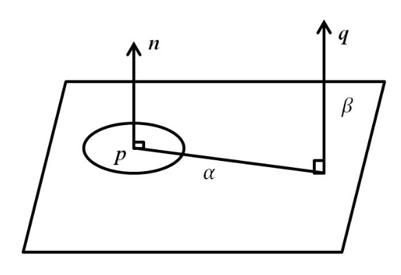
spin image방법은 feature를 ($\alpha$,$\beta$)로 나타내고 point p 주변의 neighboring point q에 대해서 다음과 같이 나타낸다. $\alpha=n_q\cdot(p-q), \beta=\sqrt{ {\Vert p-q\Vert}^2 - \alpha^2}$ 이것은 결국 p에 대해서 q를 surface plane과 parallel한 방향으로의 거리 surface normal과 parallel한 방향으로의 거리를 구한 것이다.
spin image는 주변의 모든 neighboring point에 대해서 $(\alpha, \beta)$ 를 구해서 2D discrete bin안에 넣는 것으로 구할 수 있다. 이것이 spin image인 이유는 결국 surface normal vector 부터 시작하는 half-plane을 정의하면 이를 surface normal을 기준으로 한 바퀴 돌리는 동안 이 half-plane상에 neighbor point가 위치한 지점마다 point를 찍어서 만든 이미지가 되기 때문인것 같다.
이 descriptor는 occlusion이나 clutter에 대해선 robust하지만 high-level noise에 대해서 취약하다고 한다.
2. 3D Shape Context (3DSC) - 3D object recognition
Paper: Recognizing Objects in Range Data Using Regional Point Descriptors

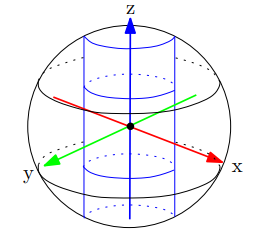
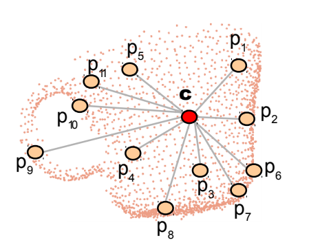
3D shape context는 2D shape context descriptor를 3D로 확장시킨 방법이다. 주어진 point p를 중심으로 한 spherical support region에서 north pole의 방향을 surface normal의 방향으로 정하고 3D bin을 azimuth angle과 elevation angle을 동일하게 나누고 반지름의 간격은 logarithmical하게 나눈 형태이다. 최종적으로 3DSC의 feature형태는 저렇게 나눈 3D bin안에 들어있는 point의 weighted sum으로써 나타내게 된다. 즉, point p 주변의 local shape를 나타낸 것이다. 그러나 이 방법은 각각의 feature point마다 reference frame이 없기 때문에 feature를 사용할 때 computation양이 많다고 한다.
3. Eigenvalues Based Descriptors - 3D terrain classification
Paper: Natural terrain classification using 3-d ladar data
Eigenvalues based descriptor는 saliency feature를 뽑아내는 방법이다. Eigenvalue는 point p 주변의 local support region 내부에 있는 neighboring points의 co-variance matrix를 decomposition해서 얻고 이 eigenvalue를 내림 차순으로 $\lambda_0 \geq \lambda_1 \geq \lambda_2$ 정의한다.
scattered된 point에 대해서는 dominant한 direction이 없기 때문에 $\lambda_0 \simeq \lambda_1 \simeq \lambda_2$ 가 될 것이고 linear structure라면 principal direction이 plane위에 생기므로 $\lambda_0,\lambda_1 \gg \lambda_2$ 의 형태가 되고 surface 경우라면 principal direction이 surface normal과 나란해지므로 $\lambda_0 \gg \lambda_1,\lambda_2$ 의 형태가 된다.
위의 사실들을 바탕으로 eigenvalue의 linear combination을 이용해 saliencies를 구하면 다음과 같이 된다.
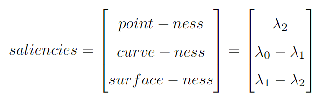
$\lambda_2$ 가 크다는 것은 결국 dominant한 direction이 없다는 것이기에 scatter의 형태에 가깝다는 얘기고 작다는 것은 dominant한 direction들이 있다는 것이고 이는 line이든 surface든 어떤 형태를 이루기 때문에 point-ness가 작다고 말할 수 있다.
$\lambda_0 - \lambda_1$ 이 크다는 것은 가장 dominant한 direction으로 치우쳐져 있다는 의미이고 이는 curve-ness가 크다고 말할 수 있고 $\lambda_1 - \lambda_2$ 가 크다는 것은 가장 dominant하지 않은 direction이 크기가 작다는 얘기이기 때문에 surface의 형태에 가까워지고 이는 surface-ness가 크다고 말할 수 있다.
4. Distribution Histogram (DH) - 3D segmentation
Paper: Discriminative learning of markov random fields for segmentation of 3d scan data
Distribution histogram은 각각의 point의 주변의 principal plane을 이용한다.
특정한 cube를 정의 하고 cube내에서 PCA를 사용해서 처음 두 개의 principal components를 이용해 plane을 얻고 cube를 평면방향으로 bin을 나눈다. 그래서 feature의 형태는 단순하게 이렇게 나눠진 bin안에 들어간 point의 수를 더해서 occupancy voxel grid의 형태가 된다.
5. Histogram of Normal Orientation (HNO) - 3D object classification and segmentation
Paper: Robust 3d scan point classification using associative markov networks
이 방법은 단순히 point $p$ 를 기준으로 주변의 point와의 surface normal의 angle의 차이의 cosine값을 이용하는 방법이다. 이 cosine값을 가지고 histogram을 생성한다.
만약 curvature가 심하면 histogram은 uniformly distributed 하게 되고 flat area에서는 뾰족한 형태의 histogram을 갖게 된다.
6. Intrinsic Shape Signatures (ISS) - 3D object recognition
Paper: Intrinsic Shape Signatures: A Shape Descriptor for 3D Object Recognition
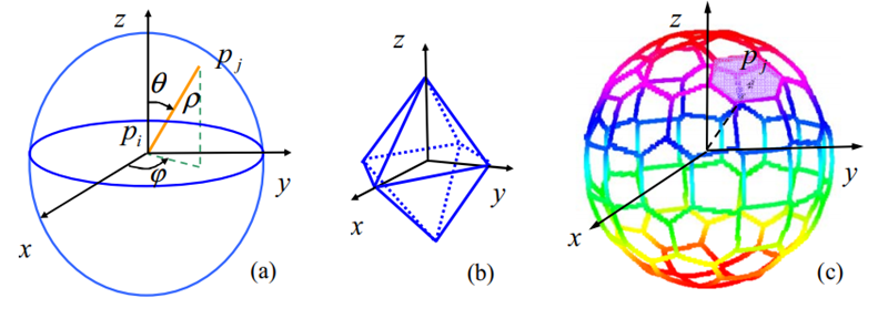
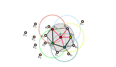
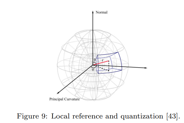
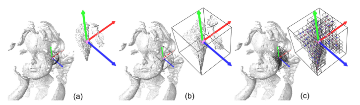
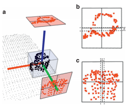
Intrinsic shape signature는 다음과 같은 방식으로 구할 수 있다. point $p$ 주변의 radius가 r인 구 내부의 point들을 이용하여 LRF(local reference frame)를 구하고 이 LRF를 이용해 bin partitioning을 한다. 여기서 cartesian partition보다 polar partition이 rotation error에 대해 더 robust 하므로 azimuth angle과 elevation angle $(\theta, \phi)$로 분할한다. 그런데 이를 균일하게 angle로만 분할을 해버리면 bin의 크기가 일정하지가 않고 pole근처에서의 성능이 저하가 되므로 다른 방식으로 분할을 한다.
LRF를 이용해 base octahedron을 정의하고 이 base octahedron의 vertex를 기준이 되는 sphere위에 projection을 시켜서 sphere위에 grid의 center를 만들고 projection된 point에 대해서 nearest center가 point가 속하게 되는 grid의 좌표$(\theta, \phi)$가 되며 grid에 속하는 point의 갯수로 feature embedding을 한다. 만약 angluar resolution을 높이고 싶으면 polyhedron에 있는 모든 triangle에 대해 순차적으로 sub triangluation을 해서 resolution을 조정한다. 위의 (c)그림은 이 sub triangulation을 3번 한 결과이다.
7. ThrIFT - 3D object recognition
Paper: Thrift: Local 3D Structure Recognition

ThrIFT는 SIFT와 SURF로 부터 아이디어를 얻어서 orientation information을 고려한 방법이다. point $p$에 대해서 window를 2개를 잡아서 $w_{small}, w_{large}$의 영역에서 각각 least-square로 plane normal $n_{small}, n_{large}$를 계산한다. feature로 만들어 지는것은 이 두 normal사이의 angle의 histogram이 된다. 이 방법은 noise에 매우 민감하다고 한다.
8. Point Feature Histogram (PFH) - 3D registration
Paper: Persistent point feature histograms for 3d point clouds
point feature histogram은 특정 영역내의 point쌍들의 관계와 surface normal을 사용해 geometric property를 나타낸 방법이다. 모든 point $p$와 그 주변의 neighbor point의 쌍에 대해서 기준 point를 $p_s$ 다른 하나를 $p_t$라 하고 $p_s$에서의 Darboux frame을 다음과 같은 식으로 정의한다.
$u = n_s$, $v=u \times {(p_t-p_s)\over{\Vert p_t-p_s\Vert}_2}$, $w=u\times v$
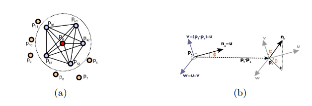
이 frame 상에서 normal $n_s, n_t$사이의 difference를 $\alpha, \Phi, \theta$ . 즉, 3개의 angular feature로 사용하고 여기다가 point pair의 distance를 feature로 사용한다.
PFH의 최종 형태는 이 4가지 feature의 4D-histogram bin의 형태가 된다.
9. Fast Point Feature Histogram (FPFH) - 3D registration
Paper: Fast Point Feature Histograms (FPFH) for 3D registration
FPFH는 이름에서 알 수 있듯이 위의 PFH에서 time complexity를 줄이기 위해서 simplifying한 방법이라고 생각하면 된다. 기존의 PFH의 time complexity는 $k$개의 neighbor를 사용할때 $o(nk^2)$인데 FPFH는 $o(nk)$의 time complexity를 가지는 알고리즘이다. FPFH는 2개의 step으로 나뉘는데 SPFH(simplified point feature histogram)을 구하는 과정과 point마다 구한 SPFH를 기준이되는 query point와 neighboring point의 SPFH를 weighted sum 해서 구하는 step으로 나뉜다.
첫번째 step은 PFH를 구하는 법과 유사한데 PFH가 $\alpha, \Phi, \theta$ , $d$의 값을 가지는 4D space상의 histogram이라면 SPFH는 단순히 $\alpha, \Phi, \theta$ 에 대해서 각각 1D histogram을 만들고 concatenate하는 식으로 구성한다.
두번째 step은 query point의 SPFH와 주변 point들의 SPFH의 weighted sum을 해서 최종 FPFH를 구한다. 식은 아래와 같다.
$FPFH(p_q)=SPFH(p_q)+{1\over k}\sum_{i=1}^k w_k \cdot SPFH(p_k)$
여기서 $w_k={1\over\sqrt{exp{\Vert p_q - p_k\Vert }}}$ 로 query point과 neighbor 사이의 distance를 반영하는 weight 이다.
10. Radius-based Surface Descriptor (RSD)
Paper: General 3D modelling of novel objects from a single view
RSD는 주변 point와의 radial relation을 계산하여 geometric property를 나타낸다고 한다. Radius는 두 point사이의 distance와 normal의 angle차이를 이용해 다음과 같이 modeling한다.
$d_\alpha = \sqrt2 r \sqrt{1-cos(\alpha)} = r\alpha + r{\alpha}^3/24 + O(\alpha^5)$
주변의 모든 point에 대해서 위의 equation을 계산하여 그 중 maximum radius와 minimum radius를 사용해 final descriptor를 얻는다. 각각 point마다 feature의 형태는 다음과 같다 $d_i =[r_{max}, r_{min}]$.

RSD의 2D histogram
이 descriptor는 결국 기준 point과 주변 point가 이루는 surface가 거대한 sphere의 일부라고 가정하고 그 sphere의 radius를 구해서 그 중 가장 작은 radius와 가장 큰 radius를 구한다는 것이다. Radius는 ideal plane의 경우 infinity가 된다.
11. Normal Aligned Radial Feature (NARF)
Paper: NARF: 3D Range Image Features for Object Recognition
NARF는 효과적으로 interest point 주변영역의 similarity를 비교하는 descriptor라고 한다.
우선 interest point를 구하는 방법은
(a) range image에서 3D distance를 이용해 background와 foreground를 구분하는 border를 찾고
(b) image에서의 모든 pixel에 대해 local neighborhood와의 curvature와 border정보를 이용해 surface score를 부여하고
(c) 모든 image pixel에 대해 dominant direction을 구하고 이 direction에 대해 다른 direction과 얼마나 다른지, 얼마나 이 point의 surface가 변화가 있는지를 이용해 interest value를 측정하고
(d) smoothing과 non-maximum suppression을 이용해 interest point를 구한다.
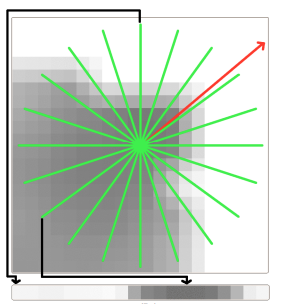
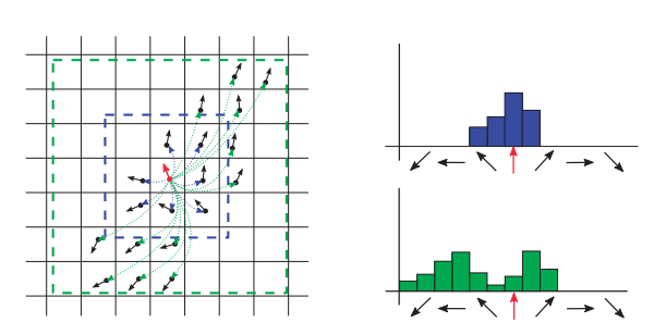
그리고 앞에서 구한 이 interest point의 주변의 normal aligned range value patch를 계산하고 이 patch에 위의 그림의 초록색 선과 같이 star pattern을 그려서 star에서의 beam이 지나는 pixel의 변화가 final descriptor의 value가 되고 unique한 orientation(빨간 화살표)을 이 descriptor로 부터 뽑아서 이 orientation을 기준으로 descriptor value들을 shift해서 rotation invariant하게 한다.
12. Signature of Histogram of Orientation (SHOT)
Paper : Efficient 3D object recognition using foveated point clouds
SHOT descriptor는 signature와 histogram의 조합이라고 보면 된다.
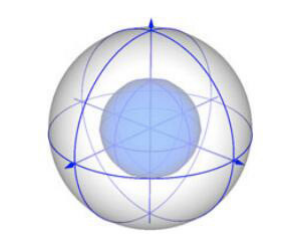
우선 feature point와 그 주변의 radius $r$내에 있는 point들의 covariance matrix에 대해서 unambiguated eigen value decompisition(EVD)을 사용해 unique하고 unambiguous한 local reference frame(LRF)을 계산한다.
그 후에 위의 그림과 같은 isotropic spherical grid를 사용해 주변 point를 $(r,\phi,\theta)$에 따라 나눠 signature structure를 정의한다. 각각의 grid영역 마다 feature point의 normal과 grid내부의 neighbodirng point들의 normal의 angle의 차이로 local histogram을 생성한다.
SHOT descriptor의 최종 형태는 모든 local histrogram을 juxtapose(concatenate?)한 형태가 된다고 한다. 여기에 texture information을 추가해 accuracy를 향상시킨 CSHOT이라는 descriptor도 있다고 한다.
13. Unique Shape Context (USC)
Paper: Unique shape context for 3D data description
USC는 3DSC에서 각각의 key point를 비교할 때 feature의 계산을 여러번하는 것을 피하기 위해서 unique, unambiguous한 local reference frame(LRF)를 추가한 3D descriptor라고 한다. query point $p$ 와 이 $p$ 주변의 radius가 $R$ 인 spherical support region에 대해서 weighted covariance $M$은 다음과 같이 정의된다.
$M=\frac{1}{Z}\sum_{i:d_i\le R}(R-d_i)(p_i-p)(p_i-p)^T$ 여기서 $Z=\sum_{i:d_i\le R}{(R-d_i)}$이다.
이 $M$은 결국 distance가 멀 수록 weight를 적게 주는 식으로 해서 query point와 주변 point사이의 covariance matrix들을 더한 형태라 말할 수 있다. LRF의 unit vector는 이 $M$을 EVD해서 얻고 여기서 나온 eigenvector와 연관된 eigenvalue의 크기에 따라 re-orient(첫번쨰와 세번째는 그대로, 두번째는 cross product의 방향)를 했다고 한다. 그래서 최종 feature는 이 LRF를 기준으로 3DSC(local descriptor 2번 참조)를 사용해서 얻는다.
14. Depth Kernel Descriptor (TODO)
Paper: Depth kernel descriptors for object recognition
kernel descriptor에서 motivation을 얻어서 만든 방법으로 3D point cloud에서 size, shape, edge들을 나타내는 5개의 local kernel descriptor를 derive 했다고 한다.
15. Spectral Histogram (SH) - 3D urban classification
Spectral histogram (SH) descriptor는 SHOT과 Eigenvalues Based Descriptor(EBD)를 합친 방법이다. point p 주변의 radius 내부의 영역의 점들에 대한 covariance matrix를 EVD해서 eigenvalue들을 구하고 크기에 따라서 $\lambda_0 \le \lambda_1 \le \lambda_2$ 순서로 정렬하고
$\lambda’_i = \lambda_i / \lambda_2$로 normalize를 한다. 그 후에 EBD처럼 $\lambda_0’, \lambda_1’-\lambda_0’, \lambda_2’ - \lambda_1’$의 값을 계산한다. 그 후에 SHOT처럼 위의 그림과 같이 영역을 나눠서 영역 안에 있는 point들에 대해서 앞에 계산한 3개의 feature를 이용해 histogram을 만든다.
16. Covariance Based Descriptors - 3D classification
Paper: Compact covariance descriptors in 3D point clouds for object recognition
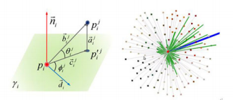
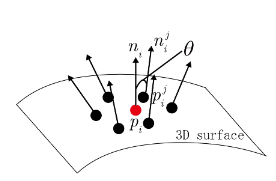
spin image로부터 발전한 방법으로 compact하고 flexible한 representation power가 큰 feature들을 많이 갖고 잇는 descriptor라고 한다. 이 descriptor가 사용하는 geometric relation은 아래의 그림에서의 $\alpha, \beta, \theta,\rho, \psi, n’$이다.
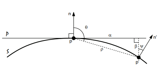
$\alpha, \beta$는 spin image에서와 같고 $\theta$는 $p$의 surface normal $n$과 $p’-p$가 이루는 각도이고 $\rho$는 $p$와 $p’$사이의 distance, $\psi$는 $p$의 surface normal $n$과 $p’$의 surface normal $n’$이 이루는 각도이다.
이 방법은 computation이 적고 memory도 적게 사용하고 tuning할 parameter가 필요 없다고 한다. 여기에 r, g, b color를 사용해서 성능을 향상 시켜보려는 시도도 있었고 shape feature와 visual feature를 함축하는 covatiance descriptor를 사용했던 시도도 있다고 한다.
17. Surface Entropy - 3D place recognition
Paper: SURE: Surface Entropy for Distinctive 3D Features
surface entropy는 shape와 color(가능한경우) information을 이용한 local shape-texture descriptor이다.
Descriptor에서 feature를 얻는 과정은 우선 surface entropy를 구해서 entropy가 특정 threshold보다 낮은 interest point들을 찾아서 noise인 point를 최대한 제거한다. 그리고 interest point $p$와 neighbor $q$에서의 surfels $(p,n_p), (q, n_q)$를 이용해 local reference frame $(u, v, w)$를 정의한다. 이 값들을 이용해 두 surfel pair의 관계를 다음과 같이 $\alpha, \beta, \gamma, \delta$로 나타낸다.
$\alpha:=arctan(2(w\cdot n_q, u\cdot n_q)), \beta:=v\cdot n_q, \gamma:=u\cdot \frac{d}{\Vert d\Vert _2}, \delta:=\Vert d\Vert_2$
최종 histogram의 형태는 모든 surfel pair에 대해서 위의 값들을 binning한 형태가 된다. 만약 color 정보를 사용할 수 있다면 HSL color space 기반으로 hue값과 saturation여부를 이용해 두개의 histogram을 더 사용하게 된다. 이 descriptor는 view-pose invariant하다.
18. 3D Self-Similarity Descriptor
Paper: Point cloud matching based on 3D self-similarity
이 descriptor는 self-similarity라는 개념을 3D point cloud로 확장해서 만든 descriptor라고 한다. self-similarity란 해당 부분의 data가 다른 부분의 data와 얼마나 닮았는지를 비교하는 property라고 한다.
3D self-similarity descriptor는 크게 두가지 단계로 나뉜다. 첫번째 단계에서 두 point사이의 normal similarity, curvature similarity, photometric similarity 이 세가지 similarity를 계산한다.
normal similarity: $s(x, y, f_{normal})=[\pi-cos^{-1}(n(x)-n(y))]/\pi$
curvature similarity: $s(x,y,f_{curv})=1-|f_{curv}(x)-f_{curv}(y)|$
photometric similarity: $1-|I(x)-I(y)|$
그리고 세개의 similarity들을 하나로 합쳐서 united similarity를 정의한다.
united similarity: $s(x,y)=\sum_{p\in PropertySet} w_p\cdot s(x, y, f_p)$
이 united similarity를 비교함으로써 self-similarity surface를 만들게 되는 것이다.
다음 단계에서는 point를 기준으로 LRF를 구해서 rotation invariant하게 하고 주변의 space를 spherical coordinate에서 quantization을 하고 각각의 bin에 존재하는 주변 point들의 average similarity값을 bin의 값으로 부여하는 식으로 descriptor를 생성한다.
이 descriptor는 distinctive geometric signature를 잘 나타낸다고 논문에서 말한다.
19. Geometric and Photometric Local Feature (GPLF)
Paper: Robust descriptors for 3D point clouds using Geometric and Photometric Local Feature
GPLF는 $f=(\alpha, \delta, \phi, \theta)$로 표현되는 geometric property들과 photometric characteristic을 온전하게 사용하여 나타낸 descriptor라고 한다.
기준 point $p$와 $p$의 normal $n$에 대해 $k$-nearest neighbor $p_i$를 구하고 이 point들을 이용해 몇개의 geometric parameter들을 다음과 같이 유도할 수 있다. $a, b, c$ 식에서 보면 알 수 있지만 $p_i$의 normal 방향을 기준으로 $p$와 $p_i$의 위치관계를 parallel, directly, perpendicular 하게 나타낸 property들이다.
\[b_i=p-p_i, \ a_i=n_i(n_i\cdot b_i), \ c_i=b_i-a_i\]우선 color feature인 $\alpha, \delta$는 HSV color space에서 아래와 같은 식을 이용해 구한다. 아래에 $h, v$는 HSV에서의 hue와 value를 의미한다. $\delta$는 식을 보면 주변 point와의 normal 기준으로 perpendicular distance와 value값의 차이의 비율을 의미한다. 즉 얼마나 색변화가 심한가를 의미하는 것이다.
\[\alpha_i = h_i, \ \delta_i = \frac{v_i-v}{\Vert c_i\Vert }\]그리고 angular feature $\phi, \theta$는 다음과 같이 정의된다.
\[\phi_i = arccos(\frac{d_i\cdot c_i}{\Vert d_i\Vert \ \Vert c_i\Vert }), \ \phi_i = \begin{cases} -\phi_i \text{ if} \ n_i\cdot(d_i \times c_i) \ge 0 \\ \ \ \ \phi_i \ \ \ \ \ \ \text{ otherwise} \end{cases}\] \[\theta_i = arccos(\frac{\Vert a_i\Vert }{\Vert c_i\Vert }), \ \theta_i = \begin{cases} \ \ \ \theta_i \text{ if} \ n_i\cdot a_i \ge 0 \\ -\theta_i \ \ \text{ otherwise} \end{cases}\]여기서 $d_i = \sum_{i=1}^k(\frac{c_i}{\Vert c_i\Vert }) \delta_ie^{-\frac{\Vert e_i\Vert }{2}}$이다. $d_i$는 일종의 point $p$를 기준으로 주변 point들의 direction들의 dominant direction이라고 보면 된다. 최종 histogram 형태는 neighbor point $p_i$의 거리에 따라서 4개의 subgroup으로 나누고 각각의 subgroup안의 point들의 4개의 feature를 모두 8개의 bin으로 나눠서 총 4x4x8의 128의 크기를 가진 histogram이 된다.
20. MCOV
Paper: MCOV: A Covariance Descriptor for Fusion of Texture and Shape Features in 3D Point Clouds
MCOV는 visual 정보와 3D shape 정보를 융합한 covariance descriptor다. 주어진 point $p$와 이 point의 주변의 radius $r$ 이내의 neighborhood $p_i$에 대해서 feature selection function $\Phi(p, r)$은 다음과 같다.
\[\Phi(p,r) = \{ \phi_{p_i}, \forall p_i \ \ \text{s.t.} |p-p_i| \le r \}\]$\phi_{p_i}=(R_{p_i}, G_{p_i}, B_{p_i}, \alpha_{p_i}, \beta_{p_i}, \gamma_{p_i})$는 각 point $p_i$에서 얻은 random variable의 vector이다. 여기서 앞의 3개의 값은 $p_i$의 R,G,B값과 관련된 값이며 texture information을 포함하고자 했고 뒤의 3개의 값은 각각 $\langle n_p, (p_i-p)\rangle, \langle n_{p_i}, (p_i,-p) \rangle, \langle n_p, n_{p_i} \rangle$ 이다. $\langle \rangle$의 의미는 두 vector사이의 angle이다. 모든 feature는 scale invariance를 위해 normalized된 값을 사용한다. 주어진 point $p$에 대해서 radius $r$이내의 covariance descriptor는 다음과 같이 나타낸다.
\[C_r(\Phi(p,r))=\frac{1}{N-1}\sum^N_{i=1}(\phi_{p_i}-\mu)(\phi_{p_i}-\mu)^T\]여기서 $\mu$는 $\phi_{p_i}$의 평균 값이며 이 식은 결국 neighboring point들의 feature 값들의 correlation을 나타낸다. MCOV의 output은 결국 6x6 symmetric matrix인 이 $C_r$이다.
21. Histogram of Oriented Principal Components (HOPC)
Paper: HOPC: Histogram of Oriented Principal Components of 3D Pointclouds for Action Recognition
HOPC는 viewpoint variation과 noise의 영향을 줄이기 위해 고안된 descriptor이다.
우선 keypoint를 중심으로 PCA를 해서 eigenvector와 eigenvalue들을 구한다. 그리고 이 eigenvector들을 $regular \ m-sided \ polyhedron$으로 부터 나온 $m$ direction들에 projection하고 eigenvalue을 이용해 scale한다. 마지막으로 projected된 eigenvector를 eigenvalue의 decreasing order에 따라서 concatenate한 3xm 크기의 matrix가 HOPC descriptor의 최종형태이다.
22. Height Gradient Histogram (HGIH)
Paper: Height gradient histogram (high) for 3d scene labeling
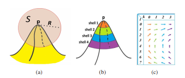
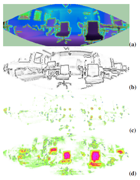
(a)는 point p의 spherical 영역을 나타내었고 (b)는 sub-region으로 나눈 예시 (c)는 각 point와 sub-region에 따른 2D histogram의 예시이다
HIGH는 $f(p)=p_x$ ($x$방향이 height)로 3D point cloud $p=(p_x, p_y, p_z)$에서 height dimension data를 추출해 활용한 descriptor라고 한다.
우선 이렇게 height 값을 추출한 후에 linear gradient reconstruction method를 사용해서 $p$에 대해 $p$주변의 point들과의 height gradient $\nabla f(p)$를 계산한다.
두 번째로 point $p$에 주변의 spherical 영역을 $K$개의 sub-region들로 나눠서 각 sub-region내부의 point들의 gradient 방향이 histogram의 형태로 변환된다.
마지막으로 이 HIGH feature descriptor는 모든 subregion의 histogram을 concatenate한 형태가 된다. 이 방법은 small object를 표현하기에는 적합하지 않다고 한다.
23. Equivalent Circumstance Surface Angle Descriptor (ECSAD)
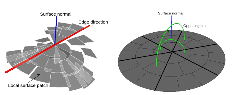
ECSAD는 3D point cloud에서 geometric edge를 찾기 위해 개발된 descriptor라고 한다. feature point $p$의 주변 region을 radial, azimuth를 축으로 몇몇 cell로 나눈다. 그리고 각각의 cell 내부의 주변 point들에 대해서 $p$에서의 normal $n$과 $p-p_i$ 사이의 angle의 평균을 구한다. 여기서 empty bin은 주변 bin을로 부터 interpolation을 이용해서 구한다. 논문에서 사용한 ECSAD의 dimension은 4개의 radial level을 사용했고 level당 azimuth을 1, 2, 3, 4로 나눠서 총 60개의 cell이 나오게 되는데 이 descriptor는 edge를 찾는것이 목적이기 때문에 center를 기준으로 opposing bin의 값을 이용을 하는데 여기서 opposing bin 해당하는 두 cell 내부의 angle의 평균을 사용함으로써 dimension이 절반이 된다. 그래서 최종적으로 ECSAD의 descriptor 크기는 30이 된다.
24. Binary SHOT (B-SHOT)
Paper: B-SHOT : A Binary Feature Descriptor for Fast and Efficient Keypoint Matching on 3D Point Clouds
B-SHOT은 이름 그대로 SHOT의 값들을 0 또는 1로 대체한 형태라고 보면 된다. Descriptor를 구성하는 과정은 SHOT와 같은 절차로 되어있으면서 5개의 possibillity를 기준으로 binary value를 결정한다고 한다. 이 기준을 설명하기에 앞서 notation을 정리하면 SHOT descriptor의 값은 ${S_0,S_1,S_2,S_3}$이고 B-SHOT으로 변환된 descriptor의 값은 ${B_0,B_1,B_2,B_3}$로 표현할 것이다. 그리고 $S_{sum} = S_0+S_1+S_2+S_3$이다.
Case A: 모든 $S_i$가 0일 경우에 모든 $B_i$ 또한 0이다.
Case B: Case A를 만족하지 않을 경우 $S_i$중 하나가 $S_{sum}$의 값의 90% 이상을 차지한다면 해당하는 $i$번째 값으로 one-hot encoding을 한다. (i.e. ${S_0,S_1,S_2,S_3}={0.85, 0.01, 0.01,0.01}$이면${B_0,B_1,B_2,B_3}={1,0,0,0}$이다.
Case C: Case A와 Case B를 만족하지 않을 경우 $S_i$들 중 두 값의 합($S_i+S_j$)이 $S_{sum}$의 90%이상일 경우 $B_i, B_j$의 값을 1로 하고 나머지 두 값을 0으로 한다.
Case D: Case A, B, C 를 만족하지 않을 경우 $S_i$들 중 세 값의 합($S_i+S_j+S_k$)이 $S_{sum}$의 90%이상일 경우 $B_i, B_j, B_k$의 값을 1로 하고 나머지 값을 0으로 한다.
Case E: 위의 어느 조건도 만족하지 않을 경우 ${B_0,B_1,B_2,B_3}={1, 1, 1, 1}$이다.
이 B-SHOT을 사용하면 SHOT에 비해 memory도 덜 사용하고 매우 빠르다고 한다.
25. Rotation, illumination, Scale Invariant Appearance and Shape Feature (RISAS)
Paper: RISAS: A Novel Rotation, Illumination, Scale Invariant Appearance and Shape Feature
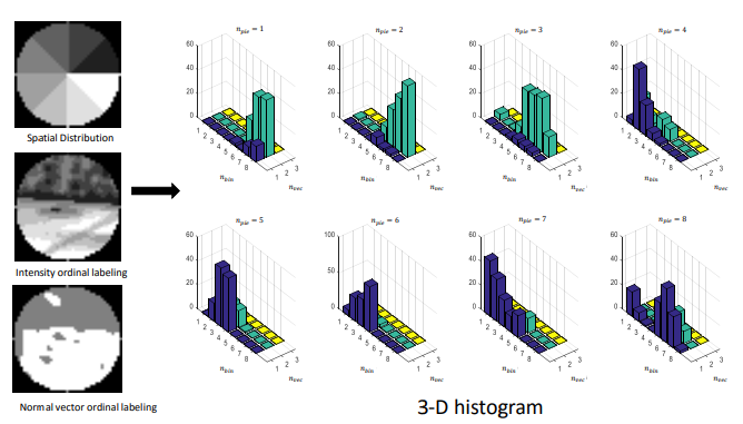
RISAS는 spatial distribution, intensity information, geometrical information의 3가지 statistical histogram을 포함한 feature vector이다.
Spatial distribution을 구하기 위해서는 spherecal support 영역을 $n_{pie}$개의 일정한 크기의 영역으로 나누고 각각의 sector안에 있는 position과 depth value를 이용해 spatial histogram을 생성한다. Sector수가 늘어날수록 descriptor가 discriminative해진다.
Intensity information은 absolute intensity대신 relative intensity를 사용해 $n_{bin}$개의 bin들로 나눠서 intensity histogram을 구성한다.
Geometric information은 기준 point $p$와 그 neiboring point $q$의 normal의 각도 차이 $\rho_i=|\langle n_p, n_q\rangle|$를 이용해 $n_{vec}$개의 bin으로 나눠서 geometric histogram을 구성한다. 여기서 대부분의 $\rho$는 1에 가까우므로 threshold $\bar{\rho}$ 이상의 값을 하나의 카테고리로 묶고 나머지를 $n_{vec}$개로 나누는 방식으로 하므로 실제로는 $n_{vec}+1$개의 bin이 된다.
최종 discriptor의 dimension은 $n_{pie} \times n_{bin} \times (n_{vec} + 1)$이 된다.
26. Colored Histograms of Spatial Concentric Surflet-Pairs (CoSPAIR)
Paper: Cospair: Colored histograms of spatial concentric surflet-pairs for 3d object recognition
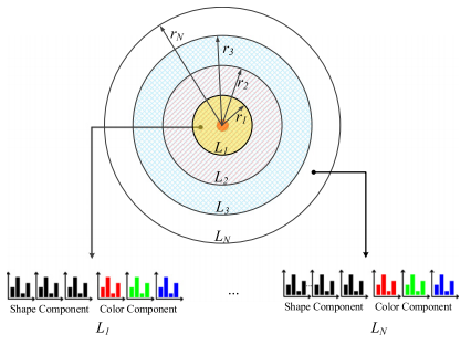
PFH와 FPFH와 유사하게 CoSPAIR는 surflet-pair relation을 기반으로 한 descriptor다.
주어진 point $p$와 그 주변 point $q$에 대해서 LRF와 세가지 angle을 구하는 법은 PFH와 같은 방법으로 구하고 radius에 따라서 spherical shell들로 영역을 나눈다.
각각의 shell에 대해서 shell 내부의 point들의 3개의 angular feature를 이용해 3개의 histogram들을 생성한다. 원래 SPAIR는 모든 shell의 histogram들을 concatenate 한다.
그런데 CoSPAIR는 마지막으로 CIELab color space의 채널들로 각각의 shell마다 histogram들을 만들고 SPAIR descriptor의 histogram들과 함께 써서 CoSPAIR를 만든다. 이 방법은 빠르고 간단한 방법이라고 알려져 있다고 한다.
27. Signature of Geometric Centroids (SGC)
Paper: Signature of geometric centroids for 3d local shape description and partial shape matching
SGC는 PCA기반으로 unique한 LRF를 중심으로한 최초의 descriptor라고 한다.
$p$의 주변의 spherical support region인 $S_p$을 LRF를 구해서 align하고 이 $S_p$를 둘러싸는 edge의 길이가 $2R$인 cubical volume을 구하고 이를 $K \times K \times K$개의 voxel로 나눈다.
마지막으로 descriptor는 이 voxel안에 들어간 point의 수와 중심 point를 기준으로 한 position을 concatenate해서 원래라면 $4 \times K \times K \times K$ dimension이어야 하지만 3개의 positional value를 $C = (Z \times L + Y)\times L + X$의 식$(L=2R)$을 통해 일종의 L-bit의 값으로 compress하여서 $2 \times K \times K \times K$로 storage공간 사용을 줄였다.
28. Local Feature Statistics Histograms (LFSH) - 3D registration
Paper: A fast and robust local descriptor for 3D point cloud registration
Local feature statistics histogram은 3개의 local shape geometry 이용해 feature를 추출하는 방식이다. Local shape geometry는 local depth, point density, angles between normals의 3가지 feature로 구성되어 있다.
point $p$ 를 중심으로한 반지름이 $r$ 인 sphere 내부에 속하는 point들을 neighboring point $p_i$ 라 하고 이 sphere에 접하고 normal vector가 $p$ 의 surface normal 인 plane을 L이라고 하고 $p_i$ 를 $L$에 projection 시킨 point 들을 ${p_i}’$ 이라고 하면 feature는 다음과 같이 구할 수 있다.
- local depth: $d = r - n \cdot ({p_i}’- p_i)$
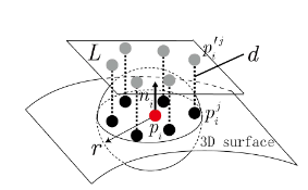
- deviation angle between normals: $\theta = arccos(n_{p’}, n_p)$
- point density: $\rho = \sqrt{ {\Vert p’ - {p_i}’\Vert}^2 - (n \cdot (p’ - {p_i}’))^2}$
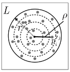
local depth 는 결국 point $p$ 의 depth를 기준으로 즉, 0으로 한 neighboring point의 depth라고 볼 수 있고 deviation angle between normal 는 말 그대로 neighboring point와 기준 point 사이의 normal vector의 angle의 차이를 구하는 것이고 point density 는 plane L상에 projection된 point들의 horizontal한 거리를 나타낸 것으로 horizontal distance를 사용해서 histogram에서 normalization을 하면 거리별로 존재할 probability를 나타내는 셈이 되고 각각의 bin의 값은 그 구간에서의 density를 표현하게 된다.
feature histogram의 최종 형태는 이 3개의 feature의 sub-histogram을 concatenation한 형태가 되며 이 방식은 low dimension을 가지며 computational complexity가 낮고 여러 nuisance에 robust하다고 한다.
29. 3D Histogram of Point Distribution (3DHoPD)
Paper: 3DHoPD: A Fast Low Dimensional 3D Descriptor
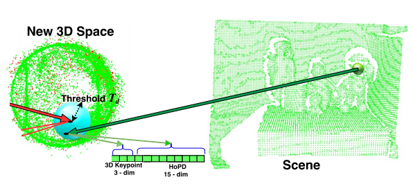
3DHoPD는 다음과 같은 과정을 통해 descriptor를 구성한다.
우선 기준 point에 대해서 rotational invariance를 위해 LRF를 구하고 이를 기준으로 align한다. 다음은 $x$축을 기준으로 $x$의 최솟값과 최댓값사이의 범위를 D개의 bin으로 나눠서 histogram들을 만들고 각각의 bin에 해당하는 point들을 넣는다. $y, z$에 대해서도 같은 방식으로 한다. 3DHoPD는 이 histogram들과 기준 point의 좌표를 concatenate해서 만든다. 이 방법의 장점은 computation이 빠르다는 것이다.
Global Descriptor
Global descriptor는 전체 3D scene에서의 geometric information을 표현하는 방법이다. local descriptor에 비해서 상대적으로 computation량이 적고 memory 사용량도 적은 편이다. 주로 object recognition, shape retrieval에 쓰인다고 한다.
1. Point Pair Feature (PPF)
Paper: Model globally, match locally: Efficient and robust 3d object recognition
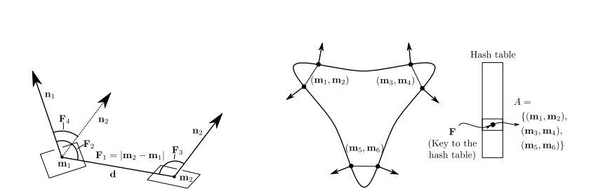
Surflet-pair feature와 유사하게 주어진 두 point $p_1, p_2$와 그 normal을 $n_1, n_2$라 하면 PPF는 다음과 같이 정의된다.
\[F=(\Vert p_1-p_2\Vert _2,\angle(n_1, p_2-p_1),\angle(n_2,p_2-p_1),\angle(n_1, n_2))\]여기서 각의 범위는 $[0,\pi]$이다. feature를 discretize하고 비슷한 값을 가진 point pair는 위의 우측의 그림과 같이 서로 합쳐서 저장한다. 이 global descriptor의 최종형태는 이렇게 PPF space의 값들을 mapping한 형태가 된다.
2. Global RSD (GRSD)
Paper: Hierarchical Object Geometric Categorization and Appearance Classification for Mobile Manipulation
GRSD는 local RSD descriptor의 global version이라고 보면 된다. Input point cloud를 voxelize하고 나서 5개의 surface primitive중 하나로 labeled된 voxel의 smallest, largest radius를 각각 구한다. 그리고 이 annotated된 voxel들의 relationship을 이용해서 특정한 task를 수행할 수 있다고 한다.
3. Viewpoint Feature Histogram (VFH)
Paper: fast 3d recognition and pose using the viewpoint feature histogram
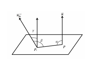
VFH는 FPFH에서 추가적으로 viewpoint variance를 고려한 방법이라고 한다. VFH는 viewpoint direction component와 surface shape component로 구성된다.
Viewpoint direction component는 central viewpoint direction과 각각 point의 surface normal의 angle difference $\beta = arcccos(n_p\cdot (v-p) / ({\Vert v-p\Vert}_2))$ 의 histogram의 형태이고,
Shape component는 FPFH처럼 centroid point기준으로 모든 point 와의 $\alpha, \phi, \theta$ angle을 각각 45개의 bin갯수를 가진 3개의 sub histogram으로 나타낸 형태이다.
VFH는 $O(n)$의 complexity를 가지며 recognition에서 높은 performance를 보이지만 noise와 occlusion에 취약했다.
4. Clustered Viewpoint Feature Histogram (CVFH)
Paper: CAD-model recognition and 6DOF pose estimation using 3D cues

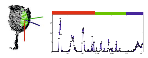
CVFH는 VFH의 확장버전이라고 보면 되는데 high curvature를 가진 point를 제거하고서 region growing algorithm을 사용함으로써 얻은 stable object region을 사용해서 이를 개선하려고 했다고 한다. Region set $S$ 에 대해서 region $s_i$가 있다고 하면 $s_i$에 대해서 FPH에서 처럼 centroid $p_c$ , normal $n_c$를 이용해서 darvoux frame$(u_i,v_i,w_i)$을 생성한다. 그리고 VFH에서 처럼 region마다 centroid를 기준으로 angular information $(\alpha, \phi, \theta, \beta)$을 4개의 histogram에 binning하고 여기에 Shape Distribution Component (SDC)를 계산한다. SDC를 계산하는 식은 다음과 같다. $SDC= \frac{(p_c-p_i)^2}{max((p_c-p_i)^2)}$ 그래서 CVFH descriptor의 최종 형태는 5개의 histogram$(\alpha, \phi, SDC, \theta, \beta)$을 concatenate해서 각각 45, 45, 45, 45, 128 dimension을 가지고 있으므로 dimension이 308인 histogram이 된다. CVFH는 좋은 성능을 내긴 하지만 euclidean space에 대한 정보가 없어서 feature에 적절한 spatial description이 포함되지 않을 수 있다고 한다.
5. Oriented, Unique and Repeatable Clustered Viewpoint Feature Histogram (OUR-CVFH)
OUR-CVFH는 CVFH와 같이 surface shape distribution component와 viewpoint component를 사용하지만 viewpoint component의 dimension을 64로 줄였다고 한다. 거기에다가 CVFH의 shape distribution component를 대체하여 surface에 있는 point들과 centroid사이의 distance의 값을 사용해 원래의 $xyz$-axis를 SGURF로 구한 RF에 align하고 $(x^-,y^-,z^-)…(x^+,y^-,z^-)…(x^+,y^+,z^+)$의 영역으로 point들을 나눠서 이 point들의 distance를 이용해 bin size가 13인 8개의 histogram들을 추가했다고 한다. OUR-CVFH의 최종 형태는 $45\times 3+13\times 8 + 64=303$ dimension의 concatenate된 histogram이다.
6. Global Structure Histograms (GSH)
Paper: Improving Generalization for 3D Object Categorization with Global Structure Histograms
GSH는 point cloud의 global, structural property를 나타내는 descriptor이다. GSH는 3개의 stage로 나뉜다.
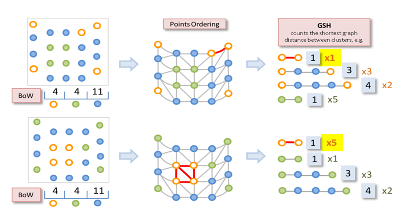
첫째는 local descriptor를 각각의 point에 적용한뒤 k-means clustering을 사용한 후 Bag of Words model을 사용해 여러개의 surface class로 point들을 labeling한다.
두번째는 object자체를 3D상의 non-empty volume을 triangulation을 통해서 surface form에 따라 다른 class들 사이의 관계를 결정한다.
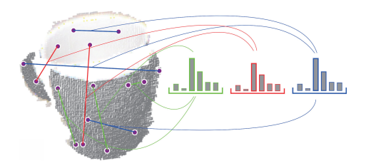
마지막으로 이전 과정에서 생성한 class들의 같은 class사이의 surface상의 shortest path의 distance로 histogram을 만들어 GSH를 만든다. 이 descriptor는 variation이 낮고 global geometry나 structure를 잘 설명한다고 한다.
7. Shape Distribution on Voxel Surfaces (SDVS)
Paper: Shape distributions on voxel surfaces for 3d object classification from depth images
Shape function이라는 개념을 기반으로 SDVS는 실제 surface에 가깝게 approximate된 voxel grid를 생성하고 임의로 sample한 두 개의 point의 distance로 두 point를 잇는 line의 location(inside, outside, mixture)에 따라서 3개의 histogram으로 binning해서 feature histogram을 생성한다. 이 방법은 간단하지만 복잡한 shape를 처리하기에는 적합하지 않다고 한다.
8. Ensemble of Shape Functions (ESF)
Paper: Ensemble of shape functions for 3D object classification
ESF는 real time application을 목표로 나온 방법론이다. ESF는 3개의 angle histogram, 3개의 area histogram, 3개의 distance histogram, 1개의 distance ratio histogram으로 이루어져 있고 각 histogram은 64개로 bin되어 총 640개의 parameter를 가지는 histogram이다.
angle, area, distance histogram은 각각 A3(sample된 3개의 point에 의해 생성된 2개의 line에 의한 angle), D3(sample된 3개의 point에 의해 생성된 area), D2(sample된 point쌍이 이루는 line의 길이) shape function의 값을 기준으로 ON, OFF, MIXED로 classifying하여 histogram을 생성한다.
D2 function에서 만들어지는 histogram ON(green), OFF(red), MIXED(blue)
D2 function에서 ON은 point들을 잇는 line이 surface위에 있을 경우, OFF는 endpoint만이 surface위에 있을 경우, MIXED는 부분적으로 ON일 경우이다.

distance ratio histogram
그리고 여기에서 line마다 ON인 부분의 ratio를 이용해 distance ratio hitogram을 구한다.

A3 fucntion에서 만들어지는 histogram
A3 fucntion에서 ON, OFF, MIXED는 angle의 맞은편의 line에 대해 D2와 같은 방식으로 classification을 한다.
D3 function에서 만들어지는 histogram
D3 function에서는 A3와 같은 방식으로 classification을 한다.
9. Global Fourier Histogram (GFH)
Paper: Performance of global descriptors for velodyne-based urban object recognition
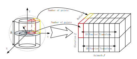
GSF는 origin이 $O$인 oriented point를 이용해 생성하는 descriptor라고 한다. global reference frame을 정하기 위해 편의상 $O$에서의 normal은 $z$-axis $(z=[0, 0,1]^T)$로 정한다. 그리고 $O$를 중심으로 한 cylindrical support region을 azimuth, radial , elevation을 균등하게 나눠서 bin을 생성한다. GFH descriptor는 각각의 bin 안에 존재하는 point 수를 합해서 생성한 3D histogram이 된다. 여기서 robustness를 증가시키기 위해서 1D FFT를 3D histogram에 적용해서 azimuth dimension에서의 frequency domain으로 transform한다. 이 descriptor는 Spin Image 방법의 단점을 보완할 수 있다고 한다.
10. Position-related Shape, Object Height along Length, Reflective Intensity Histogram (PRS, OHL and RIH)
Paper: Robust vehicle detection using 3D Lidar under complex urban environment
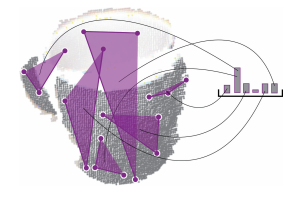
PRS, OHL and RIH는 vehicle detection rate를 크게 증가시키기 위해서 PRS, OHL, RIH라는 새로운 세가지 feature들을 사용해 vehicle과 다른 object를 robust하게 구별했다고 한다.
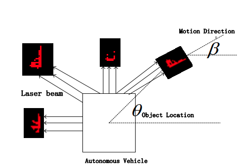
PRS는 shape feature(width-length, witdth-height ratio)와 position information(distance, orientation, angle of view)을 사용해 orientation과 angle of view에 따른 variance를 처리했다고 한다.
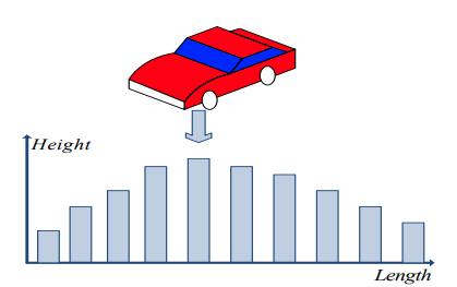
OHL은 vehicle의 bounding box를 length에 따라 몇 개의 block으로 나눠서 block들의 average height를 feature vector에 추가해서 discrimination 성능을 추가로 향상 시켰다.
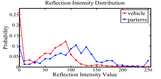
마지막으로 25개의 bin을 가진 RIH는 vehicle의 characteristic intensity distribution을 이용해 계산한다고 한다.
11. Global Orthographic Object Descriptor (GOOD)
Paper: GOOD: A global orthographic object descriptor for 3D object recognition and manipulation
GOOD는 처음에 unique하고 repeatable한 LRF를 PCA를 통해서 구한다. 그리고 point cloud를 $xy$, $yz$, $zx$ 이 세개의 plane에 orthographic하게 projection한다. 그리고 각각의 plane을 몇개의 bin들로 나누고 이 bin안에 속하는 point의 수를 세서 distribution matrix를 생성한다. 그 후에 이 matrix에 대해 entropy와 variance 이 두 가지의 statistical feature들의 distribution vector를 구한다. 이 vector들을 concatenate해서 전체 object에 대해 single vector의 형태로 feature가 나오게 된다. GOOD는 scale, pose에 대해 invariant하고 expressiveness와 computational cost 사이의 trade-off가 있다고 한다.
12. Globally Aligned Spatial Distribution (GASD) (TODO)
Paper: An Efficient Global Point Cloud Descriptor for Object Recognition and Pose Estimation
GASD는 두 가지 step으로 나뉜다. 우선 전체 model에서 PCA를 통해 RF를 구하고 이 RF에 point cloud를 align한다. 그 후에 axis-aligned된 point cloud의 bounding cube를 $m_s\times m_s \times m_s$의 cell로 나눈다. 최종 histogram은 이 각각의 grid에 들어가 있는 point의 수를 합해서 만든 histogram을 concatenate해서 얻는다. discriminative power를 증가시키기 위해서 HSV space기반의 color
13. Scale Invariant Point Feature (SIPF) (TODO)
Paper: Scale invariant point feature (SIPF) for 3D point clouds and 3D multi-scale object detection
SIPF는
14. Global Fast Point Feature Histogram (GFPFH) (TODO)
Paper: Detecting and Segmenting Objects for Mobile Manipulation
Hybrid Descriptor
1. Bottom-Up and Top-Down Descriptor (TODO)
Paper: Object Detection from Large-Scale 3D Datasets Using Bottom-Up and Top-Down Descriptors
2. Local and Global Point Feature Histogram (LGPFH) (TODO)
Paper: Real-time object classification in 3d point clouds using point feature histograms
3. Local-to-Global Signature Descriptor (LGS) (TODO)
Paper: Local-to-global signature descriptor for 3d object recognition
4. Point-Based Descriptor (TODO)
5. FPFH + VFH (TODO)
Paper: 3D Object Recognition Based on Local and Global Features Using Point Cloud Library